Data modeling techniques
This is Part 3 of a guide on migrating from PostgreSQL to ClickHouse. This content can be considered introductory, with the aim of helping users deploy an initial functional system that adheres to ClickHouse best practices. It avoids complex topics and will not result in a fully optimized schema; rather, it provides a solid foundation for users to build a production system and base their learning.
We recommend users migrating from Postgres read the guide for modeling data in ClickHouse. This guide uses the same Stack Overflow dataset and explores multiple approaches using ClickHouse features.
Partitions
Postgres users will be familiar with the concept of table partitioning for enhancing performance and manageability for large databases by dividing tables into smaller, more manageable pieces called partitions. This partitioning can be achieved using either a range on a specified column (e.g., dates), defined lists, or via hash on a key. This allows administrators to organize data based on specific criteria like date ranges or geographical locations. Partitioning helps in improving query performance by enabling faster data access through partition pruning and more efficient indexing. It also helps maintenance tasks such as backups and data purges by allowing operations on individual partitions rather than the entire table. Additionally, partitioning can significantly improve the scalability of PostgreSQL databases by distributing the load across multiple partitions.
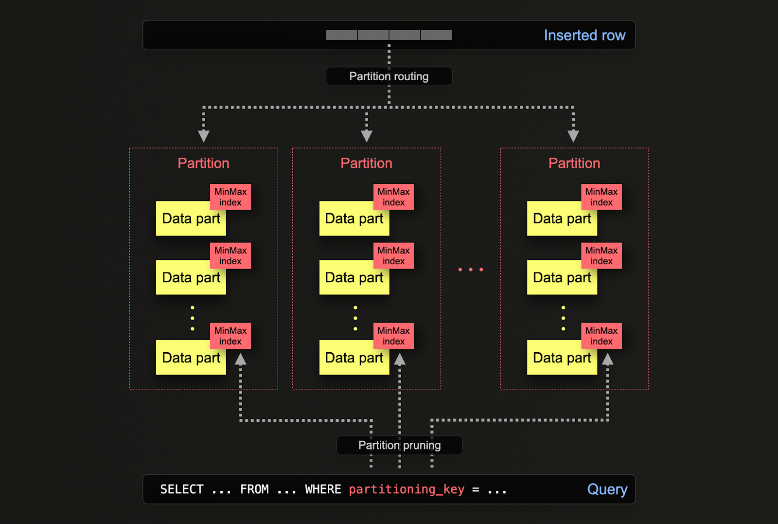
In ClickHouse, partitioning is specified on a table when it is initially defined via the PARTITION BY clause. This clause can contain a SQL expression on any columns, the results of which will define which partition a row is sent to.

The data parts are logically associated with each partition on disk and can be queried in isolation. For the example below, we partition the posts table by year using the expression toYear(CreationDate). As rows are inserted into ClickHouse, this expression will be evaluated against each row and routed to the resulting partition if it exists (if the row is the first for a year, the partition will be created).
 CREATE TABLE posts
(
	`Id` Int32 CODEC(Delta(4), ZSTD(1)),
	`PostTypeId` Enum8('Question' = 1, 'Answer' = 2, 'Wiki' = 3, 'TagWikiExcerpt' = 4, 'TagWiki' = 5, 'ModeratorNomination' = 6, 'WikiPlaceholder' = 7, 'PrivilegeWiki' = 8),
	`AcceptedAnswerId` UInt32,
	`CreationDate` DateTime64(3, 'UTC'),
...
	`ClosedDate` DateTime64(3, 'UTC')
)
ENGINE = MergeTree
ORDER BY (PostTypeId, toDate(CreationDate), CreationDate)
PARTITION BY toYear(CreationDate)
Applications of Partitions
Partitioning in ClickHouse has similar applications as in Postgres but with some subtle differences. More specifically:
- Data management - In ClickHouse, users should principally consider partitioning to be a data management feature, not a query optimization technique. By separating data logically based on a key, each partition can be operated on independently e.g. deleted. This allows users to move partitions, and thus subnets, between storage tiers efficiently on time or expire data/efficiently delete from the cluster. In example, below we remove posts from 2008.
SELECT DISTINCT partition
FROM system.parts
WHERE `table` = 'posts'

┌─partition─┐
│ 2008  	│
│ 2009  	│
│ 2010  	│
│ 2011  	│
│ 2012  	│
│ 2013  	│
│ 2014  	│
│ 2015  	│
│ 2016  	│
│ 2017  	│
│ 2018  	│
│ 2019  	│
│ 2020  	│
│ 2021  	│
│ 2022  	│
│ 2023  	│
│ 2024  	│
└───────────┘

17 rows in set. Elapsed: 0.002 sec.

	ALTER TABLE posts
	(DROP PARTITION '2008')

Ok.

0 rows in set. Elapsed: 0.103 sec.
- Query optimization - While partitions can assist with query performance, this depends heavily on the access patterns. If queries target only a few partitions (ideally one), performance can potentially improve. This is only typically useful if the partitioning key is not in the primary key and you are filtering by it. However, queries that need to cover many partitions may perform worse than if no partitioning is used (as there may possibly be more parts as a result of partitioning). The benefit of targeting a single partition will be even less pronounced to non-existence if the partitioning key is already an early entry in the primary key. Partitioning can also be used to optimize GROUP BY queries if values in each partition are unique. However, in general, users should ensure the primary key is optimized and only consider partitioning as a query optimization technique in exceptional cases where access patterns access a specific predictable subset of the day, e.g., partitioning by day, with most queries in the last day.
Recommendations for Partitions
Users should consider partitioning a data management technique. It is ideal when data needs to be expired from the cluster when operating with time series data e.g. the oldest partition can simply be dropped.
Important: Ensure your partitioning key expression does not result in a high cardinality set i.e. creating more than 100 partitions should be avoided. For example, do not partition your data by high cardinality columns such as client identifiers or names. Instead, make a client identifier or name the first column in the ORDER BY expression.
Internally, ClickHouse creates parts for inserted data. As more data is inserted, the number of parts increases. In order to prevent an excessively high number of parts, which will degrade query performance (more files to read), parts are merged together in a background asynchronous process. If the number of parts exceeds a pre-configured limit, then ClickHouse will throw an exception on insert - as a "too many parts" error. This should not happen under normal operation and only occurs if ClickHouse is misconfigured or used incorrectly e.g. many small inserts.
Since parts are created per partition in isolation, increasing the number of partitions causes the number of parts to increase i.e. it is a multiple of the number of partitions. High cardinality partitioning keys can, therefore, cause this error and should be avoided.
Materialized views vs projections
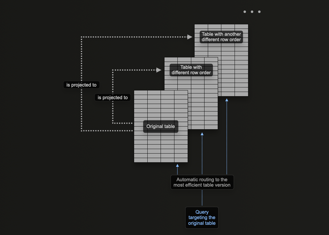
Postgres allows for the creation of multiple indices on a single table, enabling optimization for a variety of access patterns. This flexibility allows administrators and developers to tailor database performance to specific queries and operational needs. ClickHouse’s concept of projections, while not fully analogous to this, allows users to specify multiple ORDER BY clauses for a table.
In ClickHouse data modeling docs, we explore how materialized views can be used in ClickHouse to pre-compute aggregations, transform rows, and optimize queries for different access patterns.
For the latter of these, we provided an example where the materialized view sends rows to a target table with a different ordering key than the original table receiving inserts.
For example, consider the following query:
SELECT avg(Score)
FROM comments
WHERE UserId = 8592047

   ┌──────────avg(Score)─┐
1. │ 0.18181818181818182 │
   └─────────────────────┘

1 row in set. Elapsed: 0.040 sec. Processed 90.38 million rows, 361.59 MB (2.25 billion rows/s., 9.01 GB/s.)
Peak memory usage: 201.93 MiB.
This query requires all 90m rows to be scanned (admittedly quickly) as the UserId is not the ordering key. Previously, we solved this using a materialized view acting as a lookup for the PostId. The same problem can be solved with a projection. The command below adds a projection for the ORDER BY user_id.
ALTER TABLE comments ADD PROJECTION comments_user_id (
SELECT * ORDER BY UserId
)

ALTER TABLE comments MATERIALIZE PROJECTION comments_user_id
Note that we have to first create the projection and then materialize it. This latter command causes the data to be stored twice on disk in two different orders. The projection can also be defined when the data is created, as shown below, and will be automatically maintained as data is inserted.
CREATE TABLE comments
(
	`Id` UInt32,
	`PostId` UInt32,
	`Score` UInt16,
	`Text` String,
	`CreationDate` DateTime64(3, 'UTC'),
	`UserId` Int32,
	`UserDisplayName` LowCardinality(String),
	PROJECTION comments_user_id
	(
    	SELECT *
    	ORDER BY UserId
	)
)
ENGINE = MergeTree
ORDER BY PostId
If the projection is created via an ALTER, the creation is asynchronous when the MATERIALIZE PROJECTION command is issued. Users can confirm the progress of this operation with the following query, waiting for is_done=1.
SELECT
	parts_to_do,
	is_done,
	latest_fail_reason
FROM system.mutations
WHERE (`table` = 'comments') AND (command LIKE '%MATERIALIZE%')

   ┌─parts_to_do─┬─is_done─┬─latest_fail_reason─┐
1. │       	1 │   	0 │                	│
   └─────────────┴─────────┴────────────────────┘

1 row in set. Elapsed: 0.003 sec.
If we repeat the above query, we can see performance has improved significantly at the expense of additional storage.
SELECT avg(Score)
FROM comments
WHERE UserId = 8592047

   ┌──────────avg(Score)─┐
1. │ 0.18181818181818182 │
   └─────────────────────┘

1 row in set. Elapsed: 0.008 sec. Processed 16.36 thousand rows, 98.17 KB (2.15 million rows/s., 12.92 MB/s.)
Peak memory usage: 4.06 MiB.
With an EXPLAIN command, we also confirm the projection was used to serve this query:
EXPLAIN indexes = 1
SELECT avg(Score)
FROM comments
WHERE UserId = 8592047

	┌─explain─────────────────────────────────────────────┐
 1. │ Expression ((Projection + Before ORDER BY))     	│
 2. │   Aggregating                                   	│
 3. │ 	Filter                                      	│
 4. │   	ReadFromMergeTree (comments_user_id)      	│
 5. │   	Indexes:                                  	│
 6. │     	PrimaryKey                              	│
 7. │       	Keys:                                 	│
 8. │         	UserId                              	│
 9. │       	Condition: (UserId in [8592047, 8592047]) │
10. │       	Parts: 2/2                            	│
11. │       	Granules: 2/11360                     	│
	└─────────────────────────────────────────────────────┘

11 rows in set. Elapsed: 0.004 sec.
When to use projections
Projections are an appealing feature for new users as they are automatically maintained as data is inserted. Furthermore, queries can just be sent to a single table where the projections are exploited where possible to speed up the response time.

This is in contrast to materialized views, where the user has to select the appropriate optimized target table or rewrite their query, depending on the filters. This places greater emphasis on user applications and increases client-side complexity.
Despite these advantages, projections come with some inherent limitations which users should be aware of and thus should be deployed sparingly.
- Projections don't allow to use different TTL for the source table and the (hidden) target table, materialized views allow different TTLs.
- Projections don't currently support
optimize_read_in_orderfor the (hidden) target table. - Lightweight updates and deletes are not supported for tables with projections.
- Materialized views can be chained: the target table of one materialized view can be the source table of another materialized view, and so on. This is not possible with projections.
- Projections don't support joins; materialized views do.
- Projections don't support filters (WHERE clause); materialized views do.
We recommend using projections when:
- A complete reordering of the data is required. While the expression in the projection can, in theory, use a
GROUP BY,materialized views are more effective for maintaining aggregates. The query optimizer is also more likely to exploit projections that use a simple reordering, i.e.,SELECT * ORDER BY x. Users can select a subset of columns in this expression to reduce storage footprint. - Users are comfortable with the associated increase in storage footprint and overhead of writing data twice. Test the impact on insertion speed and evaluate the storage overhead.

