Migrating from BigQuery to ClickHouse Cloud
Why use ClickHouse Cloud over BigQuery?
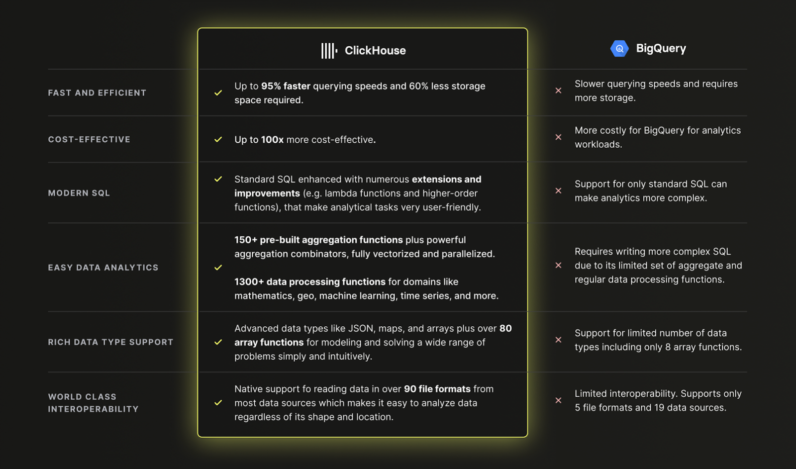
TLDR: Because ClickHouse is faster, cheaper, and more powerful than BigQuery for modern data analytics:
Loading data from BigQuery to ClickHouse Cloud
Dataset
As an example dataset to show a typical migration from BigQuery to ClickHouse Cloud, we use the Stack Overflow dataset documented here. This contains every post, vote, user, comment, and badge that has occurred on Stack Overflow from 2008 to Apr 2024. The BigQuery schema for this data is shown below:
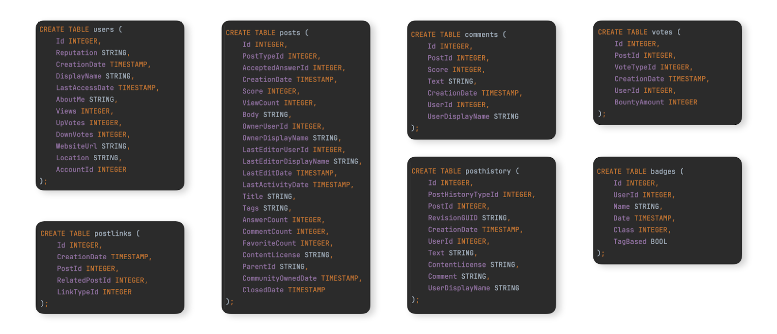
For users who wish to populate this dataset into a BigQuery instance to test migration steps, we have provided data for these tables in Parquet format in a GCS bucket and DDL commands to create and load the tables in BigQuery are available here.
Migrating data
Migrating data between BigQuery and ClickHouse Cloud falls into two primary workload types:
- Initial bulk load with periodic updates - An initial dataset must be migrated along with periodic updates at set intervals e.g. daily. Updates here are handled by resending rows that have changed - identified by either a column that can be used for comparisons (e.g., a date) or the XMIN value. Deletes are handled with a complete periodic reload of the dataset.
- Real time replication or CDC - An initial dataset must be migrated. Changes to this dataset must be reflected in ClickHouse in near-real time with only a delay of several seconds acceptable. This is effectively a Change Data Capture (CDC) process where tables in BigQuery must be synchronized with ClickHouse i.e. inserts, updates and deletes in the BigQuery table must be applied to an equivalent table in ClickHouse.
Bulk loading via Google Cloud Storage (GCS)
BigQuery supports exporting data to Google's object store (GCS). For our example data set:
-
Export the 7 tables to GCS. Commands for that are available here.
-
Import the data into ClickHouse Cloud. For that we can use the gcs table function. The DDL and import queries are available here. Note that because a ClickHouse Cloud instance consists of multiple compute nodes, instead of the
gcstable function, we are using the s3Cluster table function instead. This function also works with gcs buckets and utilizes all nodes of a ClickHouse Cloud service to load the data in parallel.
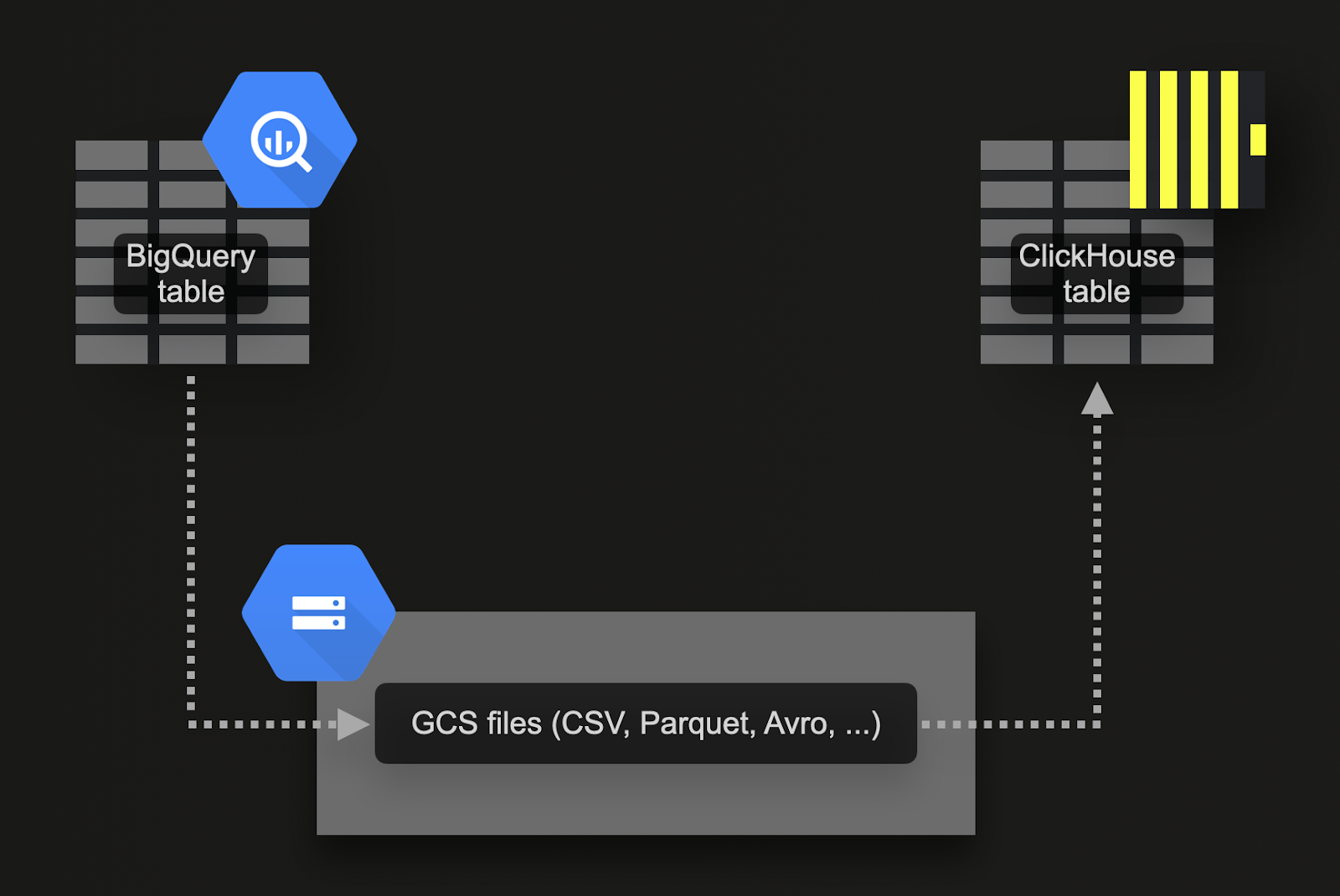
This approach has a number of advantages:
- BigQuery export functionality supports a filter for exporting a subset of data.
- BigQuery supports exporting to Parquet, Avro, JSON, and CSV formats and several compression types - all supported by ClickHouse.
- GCS supports object lifecycle management, allowing data that has been exported and imported into ClickHouse to be deleted after a specified period.
- Google allows up to 50TB per day to be exported to GCS for free. Users only pay for GCS storage.
- Exports produce multiple files automatically, limiting each to a maximum of 1GB of table data. This is beneficial to ClickHouse since it allows imports to be parallelized.
Before trying the following examples, we recommend users review the permissions required for export and locality recommendations to maximize export and import performance.
Real-time replication or CDC via scheduled queries
Change Data Capture (CDC) is the process by which tables are kept in sync between two databases. This is significantly more complex if updates and deletes are to be handled in near real-time. One approach is to simply schedule a periodic export using BigQuery's scheduled query functionality. Provided you can accept some delay in the data being inserted into ClickHouse, this approach is easy to implement and maintain. An example is given in this blog post.
Designing Schemas
The Stack Overflow dataset contains a number of related tables. We recommend focusing on migrating the primary table first. This may not necessarily be the largest table but rather the one on which you expect to receive the most analytical queries. This will allow you to familiarize yourself with the main ClickHouse concepts. This table may require remodeling as additional tables are added to fully exploit ClickHouse features and obtain optimal performance. We explore this modeling process in our Data Modeling docs.
Adhering to this principle, we focus on the main posts table. The BigQuery schema for this is shown below:
CREATE TABLE stackoverflow.posts (
    id INTEGER,
    posttypeid INTEGER,
    acceptedanswerid STRING,
    creationdate TIMESTAMP,
    score INTEGER,
    viewcount INTEGER,
    body STRING,
    owneruserid INTEGER,
    ownerdisplayname STRING,
    lasteditoruserid STRING,
    lasteditordisplayname STRING,
    lasteditdate TIMESTAMP,
    lastactivitydate TIMESTAMP,
    title STRING,
    tags STRING,
    answercount INTEGER,
    commentcount INTEGER,
    favoritecount INTEGER,
    conentlicense STRING,
    parentid STRING,
    communityowneddate TIMESTAMP,
    closeddate TIMESTAMP
);
Optimizing types
Applying the process described here results in the following schema:
CREATE TABLE stackoverflow.posts
(
   `Id` Int32,
   `PostTypeId` Enum('Question' = 1, 'Answer' = 2, 'Wiki' = 3, 'TagWikiExcerpt' = 4, 'TagWiki' = 5, 'ModeratorNomination' = 6, 'WikiPlaceholder' = 7, 'PrivilegeWiki' = 8),
   `AcceptedAnswerId` UInt32,
   `CreationDate` DateTime,
   `Score` Int32,
   `ViewCount` UInt32,
   `Body` String,
   `OwnerUserId` Int32,
   `OwnerDisplayName` String,
   `LastEditorUserId` Int32,
   `LastEditorDisplayName` String,
   `LastEditDate` DateTime,
   `LastActivityDate` DateTime,
   `Title` String,
   `Tags` String,
   `AnswerCount` UInt16,
   `CommentCount` UInt8,
   `FavoriteCount` UInt8,
   `ContentLicense`LowCardinality(String),
   `ParentId` String,
   `CommunityOwnedDate` DateTime,
   `ClosedDate` DateTime
)
ENGINE = MergeTree
ORDER BY tuple()
COMMENT 'Optimized types'
We can populate this table with a simple INSERT INTO SELECT, reading the exported data from gcs using the gcs table function. Note that on ClickHouse Cloud you can also use the gcs-compatible s3Cluster table function to parallelize the loading over multiple nodes:
INSERT INTO stackoverflow.posts SELECT * FROM gcs( 'gs://clickhouse-public-datasets/stackoverflow/parquet/posts/*.parquet', NOSIGN);
We don't retain any nulls in our new schema. The above insert converts these implicitly to default values for their respective types - 0 for integers and an empty value for strings. ClickHouse also automatically converts any numerics to their target precision.
How are ClickHouse Primary keys different?
As described here, like in BigQuery, ClickHouse doesn't enforce uniqueness for a table's primary key column values.
Similar to clustering in BigQuery, a ClickHouse table's data is stored on disk ordered by the primary key column(s). This sort order is utilized by the query optimizer to prevent resorting, minimize memory usage for joins, and enable short-circuiting for limit clauses. In contrast to BigQuery, ClickHouse automatically creates a (sparse) primary index based on the primary key column values. This index is used to speed up all queries that contain filters on the primary key columns. Specifically:
- Memory and disk efficiency are paramount to the scale at which ClickHouse is often used. Data is written to ClickHouse tables in chunks known as parts, with rules applied for merging the parts in the background. In ClickHouse, each part has its own primary index. When parts are merged, then the merged part's primary indexes are also merged. Not that these indexes are not built for each row. Instead, the primary index for a part has one index entry per group of rows - this technique is called sparse indexing.
- Sparse indexing is possible because ClickHouse stores the rows for a part on disk ordered by a specified key. Instead of directly locating single rows (like a B-Tree-based index), the sparse primary index allows it to quickly (via a binary search over index entries) identify groups of rows that could possibly match the query. The located groups of potentially matching rows are then, in parallel, streamed into the ClickHouse engine in order to find the matches. This index design allows for the primary index to be small (it completely fits into the main memory) while still significantly speeding up query execution times, especially for range queries that are typical in data analytics use cases. For more details, we recommend this in-depth guide.
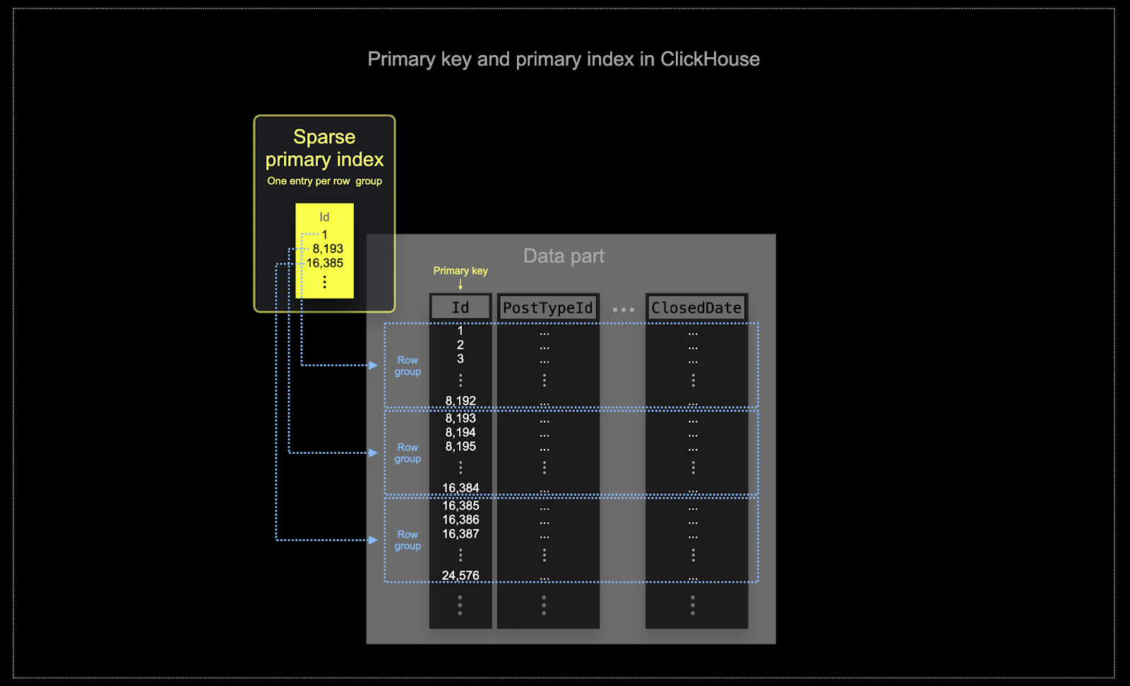
The selected primary key in ClickHouse will determine not only the index but also the order in which data is written on disk. Because of this, it can dramatically impact compression levels, which can, in turn, affect query performance. An ordering key that causes the values of most columns to be written in a contiguous order will allow the selected compression algorithm (and codecs) to compress the data more effectively.
All columns in a table will be sorted based on the value of the specified ordering key, regardless of whether they are included in the key itself. For instance, if
CreationDateis used as the key, the order of values in all other columns will correspond to the order of values in theCreationDatecolumn. Multiple ordering keys can be specified - this will order with the same semantics as anORDER BYclause in aSELECTquery.
Choosing an ordering key
For the considerations and steps in choosing an ordering key, using the posts table as an example, see here.
Data modeling techniques
We recommend users migrating from BigQuery read the guide for modeling data in ClickHouse. This guide uses the same Stack Overflow dataset and explores multiple approaches using ClickHouse features.
Partitions
BigQuery users will be familiar with the concept of table partitioning for enhancing performance and manageability for large databases by dividing tables into smaller, more manageable pieces called partitions. This partitioning can be achieved using either a range on a specified column (e.g., dates), defined lists, or via hash on a key. This allows administrators to organize data based on specific criteria like date ranges or geographical locations.
Partitioning helps with improving query performance by enabling faster data access through partition pruning and more efficient indexing. It also helps maintenance tasks such as backups and data purges by allowing operations on individual partitions rather than the entire table. Additionally, partitioning can significantly improve the scalability of BigQuery databases by distributing the load across multiple partitions.
In ClickHouse, partitioning is specified on a table when it is initially defined via the PARTITION BY clause. This clause can contain a SQL expression on any column/s, the results of which will define which partition a row is sent to.
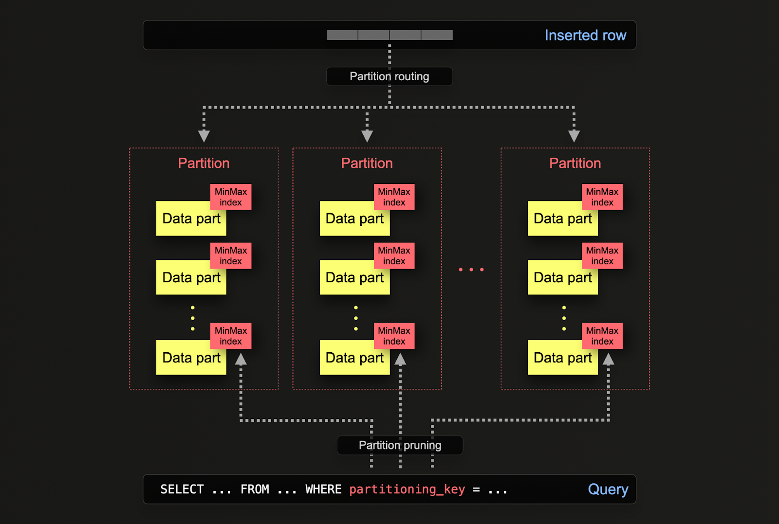
The data parts are logically associated with each partition on disk and can be queried in isolation. For the example below, we partition the posts table by year using the expression toYear(CreationDate). As rows are inserted into ClickHouse, this expression will be evaluated against each row – rows are then routed to the resulting partition in the form of new data parts belonging to that partition.
CREATE TABLE posts
(
	`Id` Int32 CODEC(Delta(4), ZSTD(1)),
	`PostTypeId` Enum8('Question' = 1, 'Answer' = 2, 'Wiki' = 3, 'TagWikiExcerpt' = 4, 'TagWiki' = 5, 'ModeratorNomination' = 6, 'WikiPlaceholder' = 7, 'PrivilegeWiki' = 8),
	`AcceptedAnswerId` UInt32,
	`CreationDate` DateTime64(3, 'UTC'),
...
	`ClosedDate` DateTime64(3, 'UTC')
)
ENGINE = MergeTree
ORDER BY (PostTypeId, toDate(CreationDate), CreationDate)
PARTITION BY toYear(CreationDate)
Applications
Partitioning in ClickHouse has similar applications as in BigQuery but with some subtle differences. More specifically:
- Data management - In ClickHouse, users should principally consider partitioning to be a data management feature, not a query optimization technique. By separating data logically based on a key, each partition can be operated on independently e.g. deleted. This allows users to move partitions, and thus subnets, between storage tiers efficiently on time or expire data/efficiently delete from the cluster. In example, below we remove posts from 2008:
SELECT DISTINCT partition
FROM system.parts
WHERE `table` = 'posts'

┌─partition─┐
│ 2008  	│
│ 2009  	│
│ 2010  	│
│ 2011  	│
│ 2012  	│
│ 2013  	│
│ 2014  	│
│ 2015  	│
│ 2016  	│
│ 2017  	│
│ 2018  	│
│ 2019  	│
│ 2020  	│
│ 2021  	│
│ 2022  	│
│ 2023  	│
│ 2024  	│
└───────────┘

17 rows in set. Elapsed: 0.002 sec.

	ALTER TABLE posts
	(DROP PARTITION '2008')

Ok.

0 rows in set. Elapsed: 0.103 sec.
- Query optimization - While partitions can assist with query performance, this depends heavily on the access patterns. If queries target only a few partitions (ideally one), performance can potentially improve. This is only typically useful if the partitioning key is not in the primary key and you are filtering by it. However, queries that need to cover many partitions may perform worse than if no partitioning is used (as there may possibly be more parts as a result of partitioning). The benefit of targeting a single partition will be even less pronounced to non-existence if the partitioning key is already an early entry in the primary key. Partitioning can also be used to optimize
GROUP BYqueries if values in each partition are unique. However, in general, users should ensure the primary key is optimized and only consider partitioning as a query optimization technique in exceptional cases where access patterns access a specific predictable subset of the day, e.g., partitioning by day, with most queries in the last day.
Recommendations
Users should consider partitioning a data management technique. It is ideal when data needs to be expired from the cluster when operating with time series data e.g. the oldest partition can simply be dropped.
Important: Ensure your partitioning key expression does not result in a high cardinality set i.e. creating more than 100 partitions should be avoided. For example, do not partition your data by high cardinality columns such as client identifiers or names. Instead, make a client identifier or name the first column in the ORDER BY expression.
Internally, ClickHouse creates parts for inserted data. As more data is inserted, the number of parts increases. In order to prevent an excessively high number of parts, which will degrade query performance (because there are more files to read), parts are merged together in a background asynchronous process. If the number of parts exceeds a pre-configured limit, then ClickHouse will throw an exception on insert as a "too many parts" error. This should not happen under normal operation and only occurs if ClickHouse is misconfigured or used incorrectly e.g. many small inserts. Since parts are created per partition in isolation, increasing the number of partitions causes the number of parts to increase i.e. it is a multiple of the number of partitions. High cardinality partitioning keys can, therefore, cause this error and should be avoided.
Materialized views vs projections
ClickHouse's concept of projections allows users to specify multiple ORDER BY clauses for a table.
In ClickHouse data modeling, we explore how materialized views can be used in ClickHouse to pre-compute aggregations, transform rows, and optimize queries for different access patterns. For the latter, we provided an example where the materialized view sends rows to a target table with a different ordering key than the original table receiving inserts.
For example, consider the following query:
SELECT avg(Score)
FROM comments
WHERE UserId = 8592047

   ┌──────────avg(Score)─┐
   │ 0.18181818181818182  │
   └────────────────────┘

1 row in set. Elapsed: 0.040 sec. Processed 90.38 million rows, 361.59 MB (2.25 billion rows/s., 9.01 GB/s.)
Peak memory usage: 201.93 MiB.
This query requires all 90m rows to be scanned (admittedly quickly) as the UserId is not the ordering key. Previously, we solved this using a materialized view acting as a lookup for the PostId. The same problem can be solved with a projection. The command below adds a projection for the ORDER BY user_id.
ALTER TABLE comments ADD PROJECTION comments_user_id (
SELECT * ORDER BY UserId
)

ALTER TABLE comments MATERIALIZE PROJECTION comments_user_id
Note that we have to first create the projection and then materialize it. This latter command causes the data to be stored twice on disk in two different orders. The projection can also be defined when the data is created, as shown below, and will be automatically maintained as data is inserted.
CREATE TABLE comments
(
	`Id` UInt32,
	`PostId` UInt32,
	`Score` UInt16,
	`Text` String,
	`CreationDate` DateTime64(3, 'UTC'),
	`UserId` Int32,
	`UserDisplayName` LowCardinality(String),
	PROJECTION comments_user_id
	(
    	SELECT *
    	ORDER BY UserId
	)
)
ENGINE = MergeTree
ORDER BY PostId
If the projection is created via an ALTER command, the creation is asynchronous when the MATERIALIZE PROJECTION command is issued. Users can confirm the progress of this operation with the following query, waiting for is_done=1.
SELECT
	parts_to_do,
	is_done,
	latest_fail_reason
FROM system.mutations
WHERE (`table` = 'comments') AND (command LIKE '%MATERIALIZE%')

   ┌─parts_to_do─┬─is_done─┬─latest_fail_reason─┐
1. │       	1 │   	0 │                	│
   └─────────────┴─────────┴────────────────────┘

1 row in set. Elapsed: 0.003 sec.
If we repeat the above query, we can see performance has improved significantly at the expense of additional storage.
SELECT avg(Score)
FROM comments
WHERE UserId = 8592047

   ┌──────────avg(Score)─┐
1. │ 0.18181818181818182 │
   └─────────────────────┘

1 row in set. Elapsed: 0.008 sec. Processed 16.36 thousand rows, 98.17 KB (2.15 million rows/s., 12.92 MB/s.)
Peak memory usage: 4.06 MiB.
With an EXPLAIN command, we also confirm the projection was used to serve this query:
EXPLAIN indexes = 1
SELECT avg(Score)
FROM comments
WHERE UserId = 8592047

	┌─explain─────────────────────────────────────────────┐
 1. │ Expression ((Projection + Before ORDER BY))     	│
 2. │   Aggregating                                   	│
 3. │ 	Filter                                      	│
 4. │   	ReadFromMergeTree (comments_user_id)      	│
 5. │   	Indexes:                                  	│
 6. │     	PrimaryKey                              	│
 7. │       	Keys:                                 	│
 8. │         	UserId                              	│
 9. │       	Condition: (UserId in [8592047, 8592047]) │
10. │       	Parts: 2/2                            	│
11. │       	Granules: 2/11360                     	│
	└─────────────────────────────────────────────────────┘

11 rows in set. Elapsed: 0.004 sec.
When to use projections
Projections are an appealing feature for new users as they are automatically maintained as data is inserted. Furthermore, queries can just be sent to a single table where the projections are exploited where possible to speed up the response time.
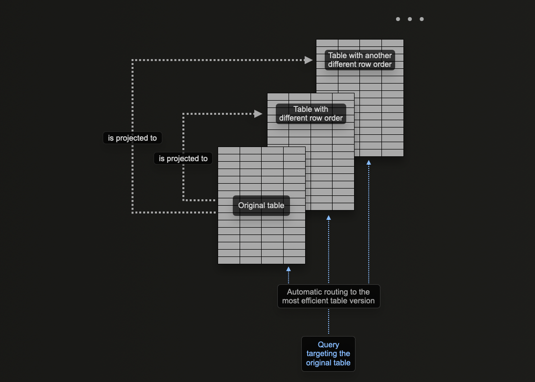
This is in contrast to materialized views, where the user has to select the appropriate optimized target table or rewrite their query, depending on the filters. This places greater emphasis on user applications and increases client-side complexity.
Despite these advantages, projections come with some inherent limitations which users should be aware of and thus should be deployed sparingly:
- Projections don't allow using different TTL for the source table and the (hidden) - target table. Materialized views allow different TTLs.
- Projections don't currently support
optimize_read_in_orderfor the (hidden) target table. - Lightweight updates and deletes are not supported for tables with projections.
- Materialized views can be chained: the target table of one materialized view can be the source table of another materialized view, and so on. This is not possible with projections.
- Projections don't support joins; materialized views do.
- Projections don't support filters (
WHEREclause); materialized views do.
We recommend using projections when:
- A complete reordering of the data is required. While the expression in the projection can, in theory, use a
GROUP BY,materialized views are more effective for maintaining aggregates. The query optimizer is also more likely to exploit projections that use a simple reordering, i.e.,SELECT * ORDER BY x. Users can select a subset of columns in this expression to reduce storage footprint. - Users are comfortable with the associated increase in storage footprint and overhead of writing data twice. Test the impact on insertion speed and evaluate the storage overhead.
Rewriting BigQuery queries in ClickHouse
The following provides example queries comparing BigQuery to ClickHouse. This list aims to demonstrate how to exploit ClickHouse features to significantly simplify queries. The examples here use the full Stack Overflow dataset (up to April 2024).
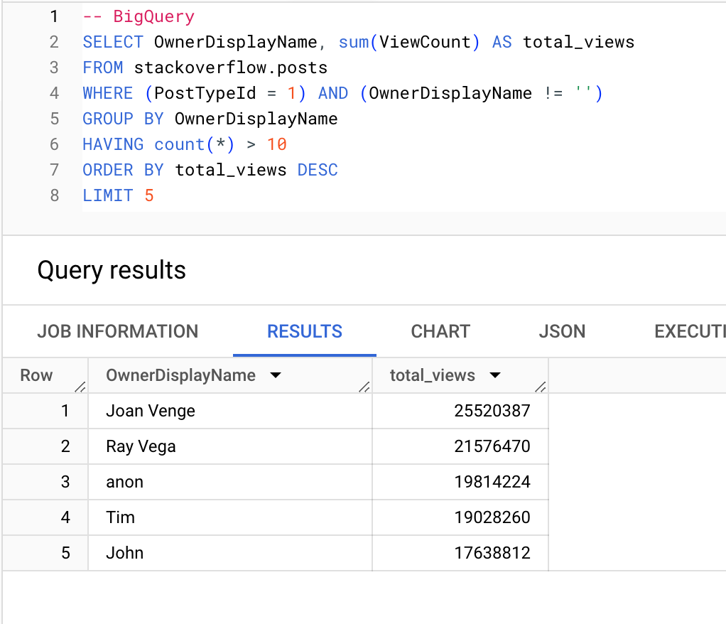
Users (with more than 10 questions) which receive the most views:
BigQuery
ClickHouse
SELECT
    OwnerDisplayName,
    sum(ViewCount) AS total_views
FROM stackoverflow.posts
WHERE (PostTypeId = 'Question') AND (OwnerDisplayName != '')
GROUP BY OwnerDisplayName
HAVING count() > 10
ORDER BY total_views DESC
LIMIT 5

   ┌─OwnerDisplayName─┬─total_views─┐
1. │ Joan Venge       │    25520387 │
2. │ Ray Vega         │    21576470 │
3. │ anon             │    19814224 │
4. │ Tim              │    19028260 │
5. │ John             │    17638812 │
   └──────────────────┴─────────────┘

5 rows in set. Elapsed: 0.076 sec. Processed 24.35 million rows, 140.21 MB (320.82 million rows/s., 1.85 GB/s.)
Peak memory usage: 323.37 MiB.
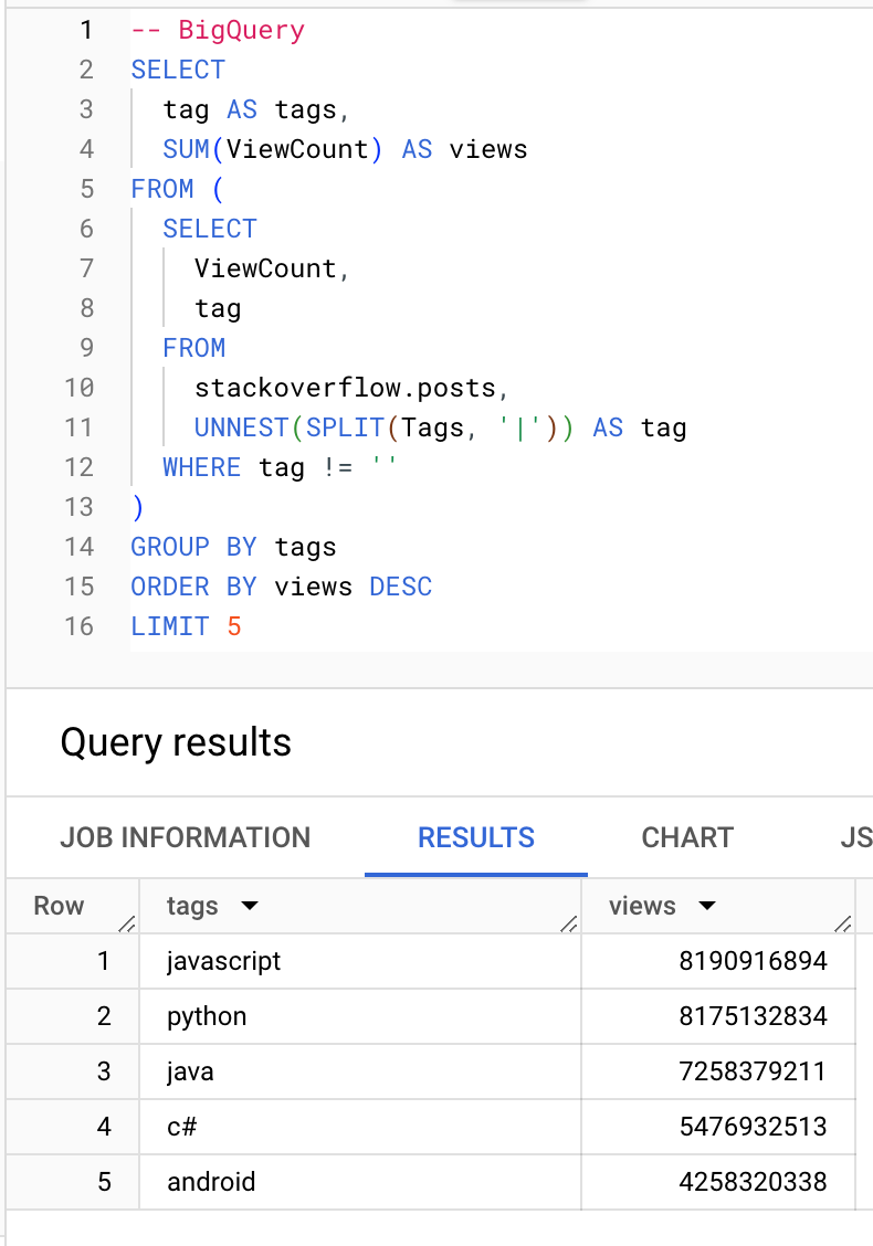
Which tags receive the most views:
BigQuery
ClickHouse
-- ClickHouse
SELECT
    arrayJoin(arrayFilter(t -> (t != ''), splitByChar('|', Tags))) AS tags,
    sum(ViewCount) AS views
FROM stackoverflow.posts
GROUP BY tags
ORDER BY views DESC
LIMIT 5


   ┌─tags───────┬──────views─┐
1. │ javascript │ 8190916894 │
2. │ python     │ 8175132834 │
3. │ java       │ 7258379211 │
4. │ c#         │ 5476932513 │
5. │ android    │ 4258320338 │
   └────────────┴────────────┘

5 rows in set. Elapsed: 0.318 sec. Processed 59.82 million rows, 1.45 GB (188.01 million rows/s., 4.54 GB/s.)
Peak memory usage: 567.41 MiB.
Aggregate functions
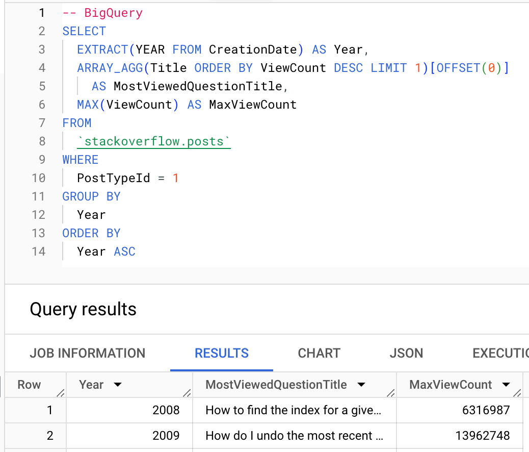
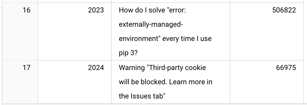
Where possible, users should exploit ClickHouse aggregate functions. Below, we show the use of the argMax function to compute the most viewed question of each year.
BigQuery
ClickHouse
-- ClickHouse
SELECT
    toYear(CreationDate) AS Year,
    argMax(Title, ViewCount) AS MostViewedQuestionTitle,
    max(ViewCount) AS MaxViewCount
FROM stackoverflow.posts
WHERE PostTypeId = 'Question'
GROUP BY Year
ORDER BY Year ASC
FORMAT Vertical


Row 1:
──────
Year:                    2008
MostViewedQuestionTitle: How to find the index for a given item in a list?
MaxViewCount:            6316987

Row 2:
──────
Year:                    2009
MostViewedQuestionTitle: How do I undo the most recent local commits in Git?
MaxViewCount:            13962748

…

Row 16:
───────
Year:                    2023
MostViewedQuestionTitle: How do I solve "error: externally-managed-environment" every time I use pip 3?
MaxViewCount:            506822

Row 17:
───────
Year:                    2024
MostViewedQuestionTitle: Warning "Third-party cookie will be blocked. Learn more in the Issues tab"
MaxViewCount:            66975

17 rows in set. Elapsed: 0.225 sec. Processed 24.35 million rows, 1.86 GB (107.99 million rows/s., 8.26 GB/s.)
Peak memory usage: 377.26 MiB.
Conditionals and Arrays
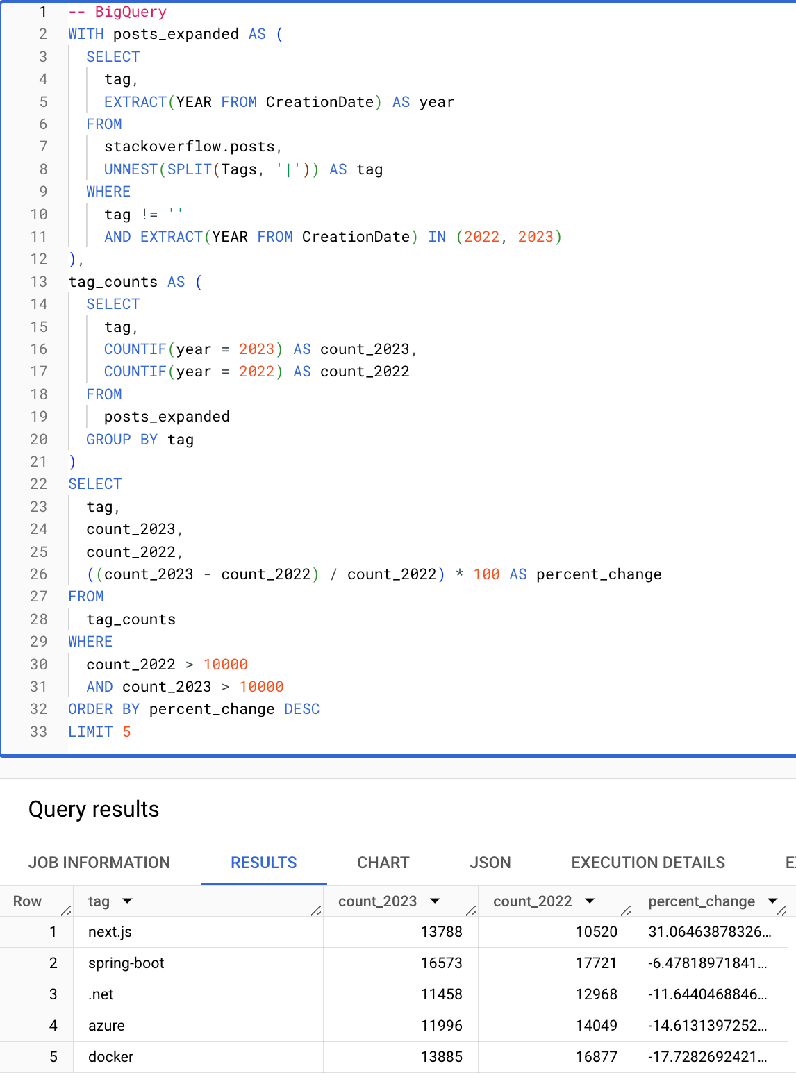
Conditional and array functions make queries significantly simpler. The following query computes the tags (with more than 10000 occurrences) with the largest percentage increase from 2022 to 2023. Note how the following ClickHouse query is succinct thanks to conditionals, array functions, and the ability to reuse aliases in the HAVING and SELECT clauses.
BigQuery
ClickHouse
SELECT
    arrayJoin(arrayFilter(t -> (t != ''), splitByChar('|', Tags))) AS tag,
    countIf(toYear(CreationDate) = 2023) AS count_2023,
    countIf(toYear(CreationDate) = 2022) AS count_2022,
    ((count_2023 - count_2022) / count_2022) * 100 AS percent_change
FROM stackoverflow.posts
WHERE toYear(CreationDate) IN (2022, 2023)
GROUP BY tag
HAVING (count_2022 > 10000) AND (count_2023 > 10000)
ORDER BY percent_change DESC
LIMIT 5

┌─tag─────────┬─count_2023─┬─count_2022─┬──────percent_change─┐
│ next.js   │   13788 │     10520 │   31.06463878326996 │
│ spring-boot │     16573 │     17721 │  -6.478189718413183 │
│ .net      │   11458 │     12968 │ -11.644046884639112 │
│ azure     │   11996 │     14049 │ -14.613139725247349 │
│ docker    │   13885 │     16877 │  -17.72826924216389 │
└─────────────┴────────────┴────────────┴─────────────────────┘

5 rows in set. Elapsed: 0.096 sec. Processed 5.08 million rows, 155.73 MB (53.10 million rows/s., 1.63 GB/s.)
Peak memory usage: 410.37 MiB.
This concludes our basic guide for users migrating from BigQuery to ClickHouse. We recommend users migrating from BigQuery read the guide for modeling data in ClickHouse to learn more about advanced ClickHouse features.

